
Validation
How well does it work?
Research prototype: not for health or regulatory decisions.
+0.88 / +0.93
NO₂ / O₃, the map's LSTM, Jan–Mar 2026. Shows it learned its target, not that it matches the air.
+0.79 / +0.93
Persistence +0.81 / +0.91
NO₂ / O₃ average at 7 and 17 monitor sites, January–March 2026.
+0.73 / +0.93
Persistence +0.68 / +0.90
NO₂ / O₃ average at 5 and 17 monitor sites, six months after training ended. Above persistence for both.
Read this first
Three kinds of evidence
Did it learn what it was taught?
Scored against its own on hours. A high score means it reproduces what it was trained on, nothing more.
Does it match real monitors on new days?
Scored against for months no model trained on (January–March and April–October 2026). Their earlier readings are in training, so this tests new times at known places, not new places.
Does it work where nothing is measured?
A cell with an EPA monitor but no measurements of its own in training: the only direct test away from instruments. One cell so far, and the model showed no skill there yet.
The story
From the first model to the current one
The first model matched its own target but not EPA monitors. Correcting its output only brought it to about zero; the big jump came from training on real EPA readings.
What each step changed
Step 0 is the original model. Step 1 keeps that model and only rescales its output per site (, fit on 2018–2025). Steps 2–5 retrain the model, each adding one change to what it learns from or is given: real EPA NO₂ in the training target, the nearest measured cell's NO₂ as an input, rolling averages, and a surface-ozone target. The dashed line is , scored on exactly the same hours.
How each change moved NO₂
How to read this chart
Taller is better. A bar at 1 would be perfect; a bar at 0 is no better than always guessing each site's usual value; a bar below 0 is worse than that guess. The dashed line is persistence (“next hour = this hour”): the bar to clear. Hover a bar for what changed at that step.
- Step 0Original modelBoundary-layer-aware target + land-use features, before any target fixes.
- Step 1Original + calibrationSame original model, output rescaled per site with a 2018–2025 fit. No retraining.
- Step 2AQS target fixReal EPA surface NO₂ blended into the training target at 11 cells.
- Step 3Spatial-lagAdds the nearest monitored cell's same-hour NO₂ as a feature.
- Step 4+ Rolling featuresAdds 3/6/12-hour rolling mean and spread of NO₂ and O₃.
- Step 5+ O₃ target fix· on the mapReplaces the O₃ target with TEMPO tropospheric O₃ + real AQS O₃. Best overall.
Where the data sits
How to read this chart
Each small square is one 10-km grid cell; darker blue means more open water. Triangles and diamonds are the instruments the model learns from. Filled circles are the EPA sites used for scoring, coloured by how well the selected model did there. Pick a model configuration on the right to see how each change moved the scores.
Orange is worse than predicting each site's average; blue beats it.
- Land → open water
- Pandora (5)
- AERONET (6)
- Ceilometer (1)
- EPA NO₂ blended into target (9)
- EPA monitor cell (scored)
Every scored cell sits on developed land. The NO₂ cells average 60% developed land and the O₃ cells 34%, against 13% for the grid. 59 of 348 cells are more than 90% open water, and none has an instrument: EPA, Pandora and AERONET sit on land, near people. These scores describe skill near monitors, not over the water.
Site by site
Where it beats the simplest forecast
Each row is one EPA site: the dot is the LSTM, the square is persistence. A line pointing right means the model wins there.
Why persistence is so hard to beat
Air quality rarely changes much in one hour, so “next hour = this hour” is already a good guess. At these sites the model is also given the monitor's current reading, so its real contribution is the margin above persistence, not the raw score.
Site by site: does the LSTM beat persistence?
How to read this chart
Each row is one EPA site. The dot is the LSTM and the square is persistence; further right is better. A coloured line from square to dot means the model beat persistence at that site; a grey one means it didn't.
Model comparison
LSTM vs simpler models
Is the neural network worth it? Four standard methods were trained on exactly the same data for comparison.
How the comparison was set up
use the same inputs, targets and date splits as the , but see only the last hour of each 24-hour window instead of the whole sequence. Gradient boosting isn't on the map; the other three are. The Taylor diagram below shows how closely each one tracks the monitors' hour-to-hour pattern.
LSTM vs simpler models on the same data
How to read this chart
Longer bars are better, on the same 0-to-1 skill scale. The dashed line is persistence, scored on the same hours. Bars that end past the line beat it; at this one-hour range, all the models land close together.
NO₂
O₃
Pattern match: correlation and variability
How to read this chart
Each dot is one model; the hollow circle marked EPA is the monitors themselves. The angle shows correlation (how well the estimates rise and fall with the real readings: further toward the bottom right is better). The distance from the corner shows how much the estimates vary compared with the readings (the solid arc is “the same amount”). The closer a dot sits to the EPA point, the better.
- LSTMr 0.918 · σ 0.88
- XGBoostr 0.926 · σ 0.85
- Gradient boostingr 0.937 · σ 0.89
- Random forestr 0.924 · σ 0.89
- Linear regressionr 0.928 · σ 0.88
- Persistencer 0.930 · σ 1.00
- Closer to the EPA point is better. The six points overlap because the models behave almost identically one hour ahead; the table has the exact values.
New data
Does it hold up six months later?
The same next-hour test on April 1 – October 5, 2026: six months that came after all training and testing.
How this test works
Each hour the models get the monitors' latest readings, prepared exactly as in training, and estimate the next hour, which they never see. Two simple guesses are scored on the same hours: and . Most of these readings come from , EPA's real-time feed, because quality-checked data take months to be published.
A mistake we caught
A one-hour misalignment inflated our scores
Our first scores compared each estimate with the wrong hour, which made them look better than they were. Every number on this site is after the fix.
What went wrong, exactly
Each estimate is for the hour after the model's last input. The original scoring compared it with the EPA reading for the input hour instead. Where the inputs contained that very reading, models were rewarded for copying it, which is why linear regression appeared to beat the LSTM. The corrected numbers were checked by an independent recomputation.
What the one-hour misalignment did
How to read this chart
Hollow circles are the scores as first reported; filled circles are the corrected ones. The longer the line between them, the more that score had been overstated by comparing each estimate with the wrong hour.
Data
When each dataset was collected
Which measurements the model learns from, which it uses as inputs, and which were tried and dropped.
Why some satellites were dropped
NO₂ and TROPOMI NO₂ were downloaded and tested as inputs, but runs with them scored worse on the test months, so they were left out. TEMPO's lower-atmosphere ozone is used only to help build the ozone training target.
Dataset coverage
How to read this chart
Each bar shows when a dataset has data, from 2018 onward; its colour shows how the model uses it. Dashed outlines are datasets that were downloaded and tested, then dropped. Scroll sideways on small screens.
Limits
What these numbers do and don't show
Downloads
Data and earlier figures
Data files
- atlas.json : every EPA-check score, per cell and model, plus site locations
- nowcast_skill.json : the April–October check, per site and month
- summary.json : map models, features and fit-to-target scores
Each chart above also has its own CSV.
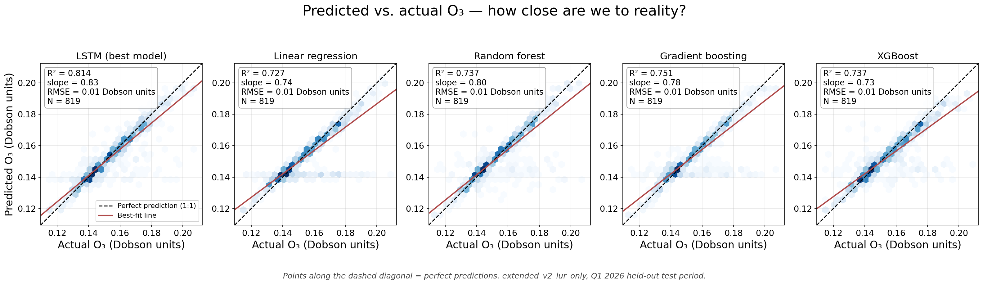
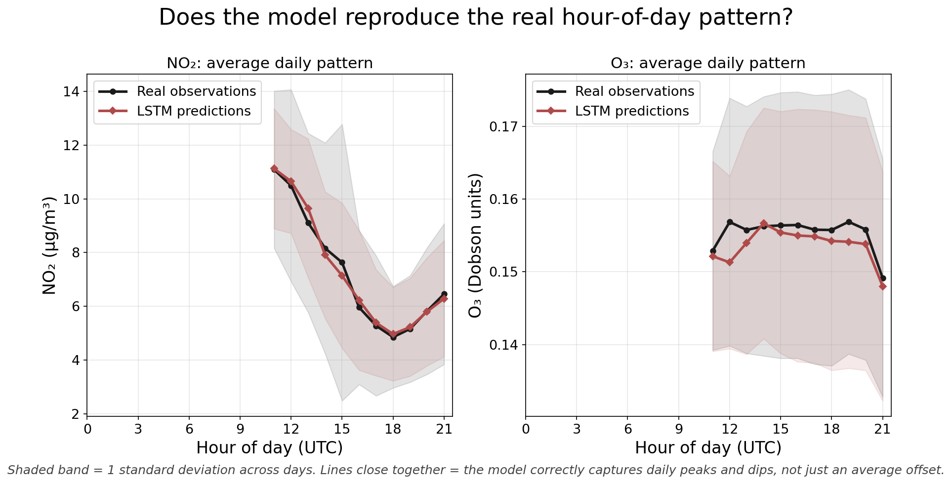
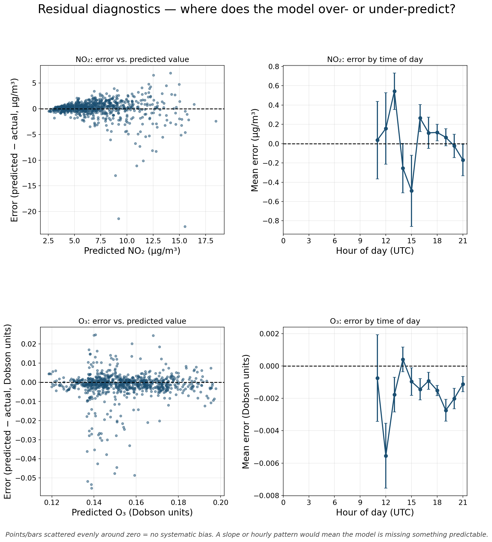
Earlier figures (original model)
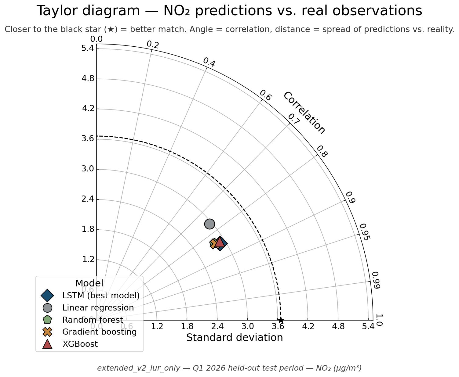
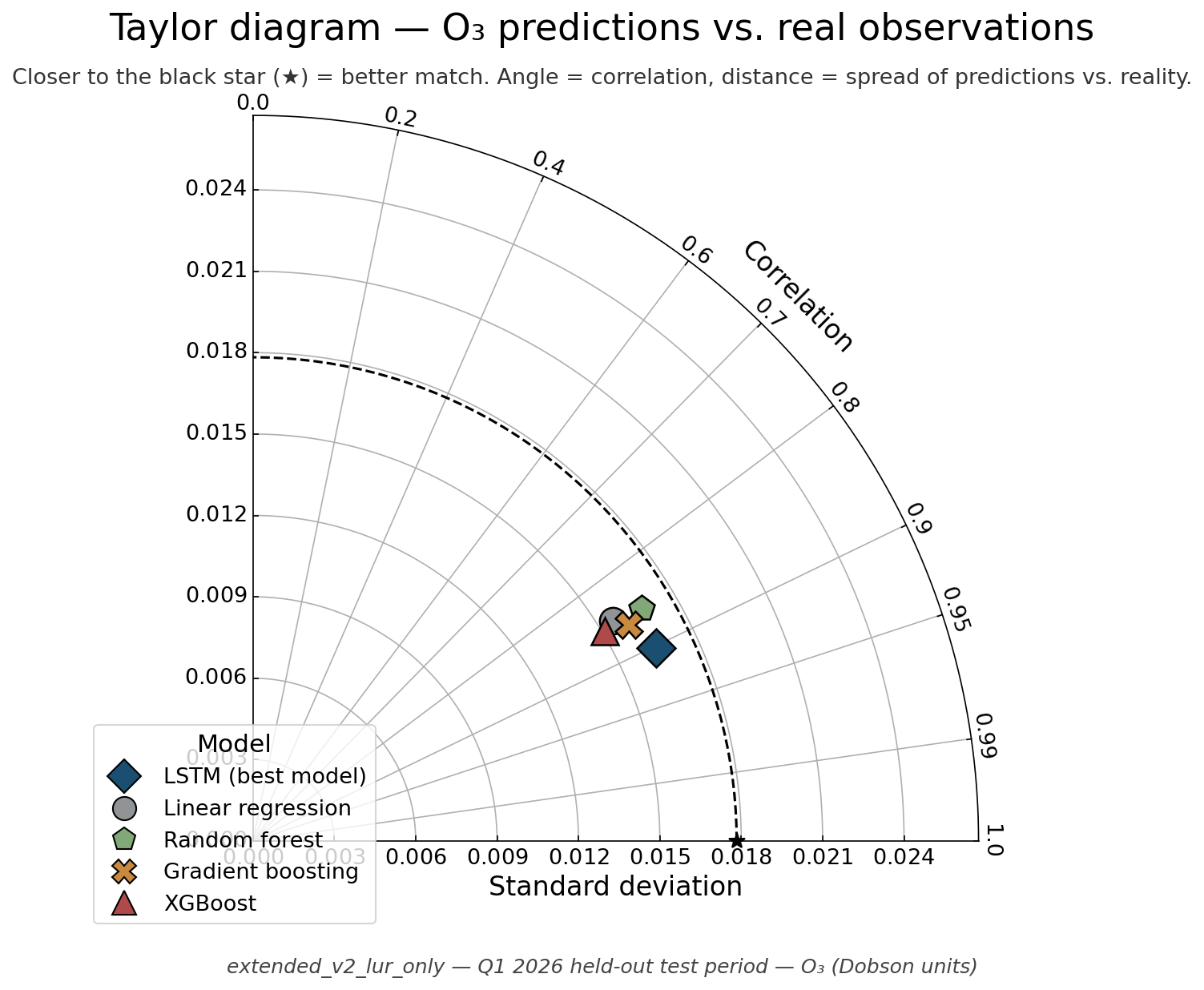
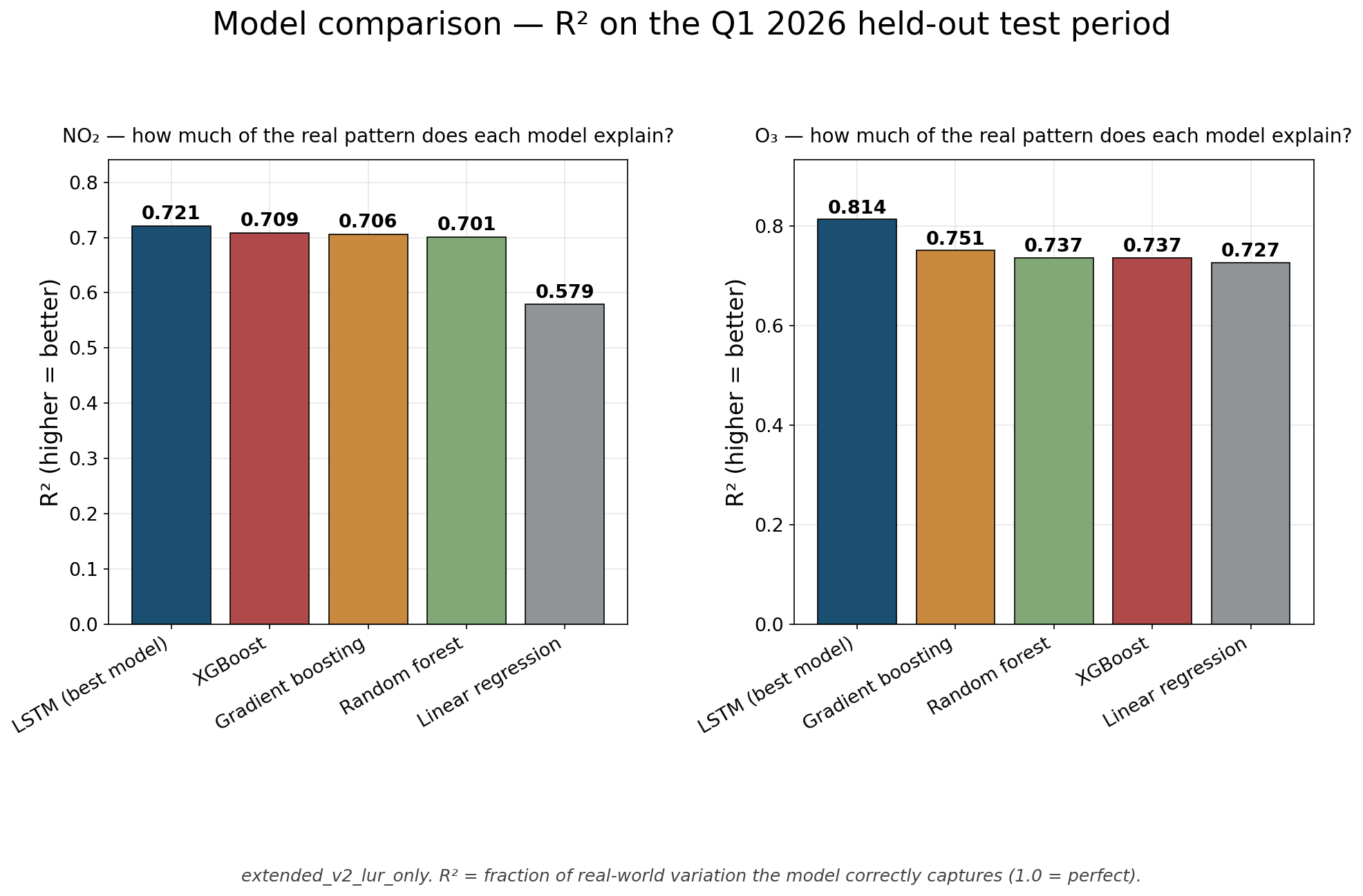
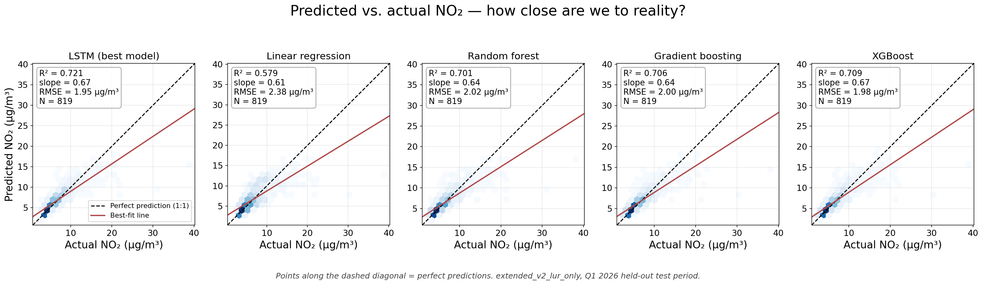
From extended_v2_lur_only, scored against its own Pandora-derived target (fit to target, not the EPA check). Its O₃ was a total column in Dobson units. Kept for the record; some of the original captions overstated the results.
Compiled Tue, 06 Oct 2026 19:46:29 GMT by scripts/build_validation_atlas_data.py and o3_target_fix/nowcast_check_apr_oct.py. See the map to explore the predictions.